Keyword & Topic Clustering For SEO With R

Keyword and topic clustering for SEO has been a hot topic for years, but one of the things I’ve noticed is that there’s been a distinct lack of discussion around how to actually do it. There’s just been a torrent of theory and a handful of (rather expensive) tools which say they’ll do it for you. With that in mind, I thought I’d spend a bit of time putting together a really basic guide using R to get you started.

I’ve been using keyword and topic clustering as part of my SEO keyword research and content planning approaches for years, also incorporating sentiment analysis and a couple of other fun areas to help my teams really target their content. While I’m not quite ready to give up all my secrets, I see so much discussion without anyone ever showing their working, doing it manually or trying to sell their tools that I wanted to help people make a bit of a start using free, open-source software.

Ready to get started? Cool.

If you’ve got some familiarity with these methodologies, feel free to skip around using the table of contents below and if you find this useful and you’d like more content like this in your inbox, please sign up for my free email newsletter.

What’s Your Email Address? *

If you are human, leave this field blank.

Δ

What You’ll Need

Before getting started, you’ll need the following things:

• Some keyword data in CSV format: Doesn’t need to be a lot and it doesn’t really matter where you got it from, you’ll just need to be aware of the column headers and edit the code accordingly. For this example, I’ve used my Google Search Console data from this site
• R: The open-source statistical language. You can get it from here
• RStudio: The best IDE for R and a lot of other languages too. You can get it from here
• The TM package for R: Packages are like plugins for the language which contain a lot of pre-built functions for specific tasks. The TM package is the best for text mining, which we’ll need to do during this process
• The Tidyverse package for R: I honestly can’t imagine a situation where I open R and don’t get Tidyverse loaded. The Tidyverse package is the definitive collection of other packages to make working with data and visualising it a lot more effective and actually fun

That’s it. You have spent precisely zero pennies to do this!

Read In Your Data

I’m going to try and be pretty thorough with this piece, but I’m also not going to be writing a step-by-step guide to using R. There’s some assumed knowledge on your part, but where required, I’ll be linking to relevant resources so you can learn more about the language and the process.

The first thing we need to do when working with any data in R is to actually read the data into our environment. After you’ve created your RStudio project, get your dataset in CSV format into your working directory and use the following command:

queries <- read.csv("Queries.csv", stringsAsFactors = FALSE)

Rename “Queries.csv” as whatever you’ve called the file with your keyword data.

Preparing Your Text Data For Clustering

Clustering is primarily a numerical function, so we’re going to need to make our text workable in a numerical world. The way we’ll do this is to turn our keywords into a Document Term Matrix using the Corpus function, and then we’ll clean that corpus up in line with best practice for text analysis.

Firstly, after reading in our data, we want to make sure that we’ve got our packages installed and live in our R environment. You can do this with the following commands:

install.packages("tm")

install.packages(“wordcloud”)

install.packages("tidyverse")

library(tm)

library(wordcloud)

library(tidyverse)

If you want to cut down on the amount of code you’re using when installing packages, you can use the combine and lapply functions like so:

instPacks <- c("tidyverse", "tm", "wordcloud")

lapply(instPacks, require, character.only = TRUE)

Now we’ve got our packages in place, we need to create that Document Term Matrix or corpus from our text. We do that with the following command:

dtm <- Corpus(VectorSource(queries$Query))

By doing this, we’ve turned our Search Console queries into a Corpus in our R environment, and it’s ready to work with. Again, adapt the “queries$Query” to whatever output you have to work with.

Cleaning a Corpus

When you’re working with text data in R, there are a few steps that you should take as standard, in order to ensure that you’re working with the most important words and also eliminating possible duplication due to capitalisation and punctuation.

I generally recommend doing the following to every corpus:

• Change all text to lower case: This brings consistency, rather than including duplicates caused by capitalisation
• Turn it to a plain-text document: This eliminates any possible rogue characters
• Remove punctuation: Eliminates duplication caused by punctuation
• Stem your words: By cutting extensions from the words in your corpus, you eliminate the duplication caused by adding “S” to some words, for example

In a lot of cases, I’d usually remove stopwords (terms such as “And”), but in this case, it’s worth keeping them since we’re going to be working with full queries rather than fragments.

Here’s how to clean that corpus up.

A Corpus-Cleaning Function For R

Functions in R are a way to make particular commands or pieces of code reproducible. Rather than entering a series of commands every time you need to use them, you can just wrap them into a function and use that function every time. They’re a time-saver and a great way to ensure that your code is easier to work with, as well as easier to share.

Based on the criteria above, here’s an R function to help you clean your keyword corpus up to prepare it for clustering your keywords:

corpusClean <- function(x){
  
  lowCase <- tm_map(x, tolower)
  
  plainText <- tm_map(lowCase, PlainTextDocument)
  
  remPunc <- tm_map(lowCase, removePunctuation)
  
  stemDoc <- tm_map(remPunc, stemDocument)
  
  output <- DocumentTermMatrix(stemDoc) 
}

Here, we’re using the TM packages’ built-in functionality to transform our corpus in the ways described above. Again, I’m not going to go into the minutiae of how this works – I don’t think I’ve got another 11k+ word post in me today – but I hope the notation is reasonably clear.

Paste this function into your R console and then we need to actually run it on our corpus. This is really easy:

corpusCleaned <- corpusClean(dtm)

We’ve created a new variable called corpusCleaned and run our function on the previous dtm variable, so we have a cleaned-up version of our original corpus. Now we’re ready to start clustering them into topics.

Using K-Means Clustering For Keywords In R

There are loads of clustering models out there that can be used for keywords – some work better than others, but the best one to start with is always the tried and trusted k-means clustering. Once you’ve done a little bit of work with this, you can explore other models, but for me, this is the best place to start.

K-means clustering is one of the most popular unsupervised machine learning models and it works by calculating the distance between different numerical vectors and grouping them accordingly.

Wikipedia is going to explain the math far better than I can, so just look at that link if you’re interested, but what we’re here to talk about today is how this can be used to cluster your search terms or target keywords into topics.

Now that we’ve cleaned up our corpus and gotten it into a state where the k-means algorithm can tokenise the terms and match them up to numeric values, we’re ready to start clustering.

Finding The Optimal Number Of Clusters

One of the biggest errors I see when people try to apply data analytics techniques to digital marketing and SEO is that they never actually make the analysis useful, they just make a pretty graph for a pitch and the actual output is never usable. That’s certainly a possible failing of topic and keyword clustering if you’re not smart about it, which is why we’re going to run through how to identify the optimal number of clusters.

There are lots of different ways that you can identify the optimal number of clusters – I’m partial to a Bayesian inference criterion, myself, although good luck getting that to run quickly in R. Since today we’re just doing an introduction, I’m going to take you through the most commonly-used way to identify the best number of topic clusters for your keywords: the Elbow Method.

The Elbow Method

The Elbow Method is probably the easiest way to find the optimal number of clusters (or k), and it’s certainly the fastest way to process it in R, but that still doesn’t mean it’s particularly quick.

Essentially, the Elbow Method computes the variance between the different terms and sees how many different clusters these could be put in up to the point that adding another cluster doesn’t provide better modelling of the data. In other words, we use this model to identify the point at which adding extra clusters becomes a waste of time. After all, if this approach doesn’t become efficient, no one will use it.

But how do we make the Elbow Method work? How do we use it to identify our target number of clusters, our k? The easiest way to do that is to visualise our clusters and take a judgement from there, hence why we installed the ggplot2 package earlier.

Running The Elbow Method In R

Before we get started, I have to say one thing: R isn’t the fastest language in the world (hence why I’m moving away from it these days) and it may take quite a while to run this process if you’ve got a large dataset. If you do have a lot of keywords, make sure you’ve got something else to do, because otherwise, you might be looking at your screen for a while.

Firstly, we need to create an empty data frame to put our cluster information into. That’s easy, we’ll just use the following command:

kFrame <- data.frame()

Now we have to use a for loop to run the clustering algorithm and put it into that data frame. This is where the processing time comes in, and I know it’s not the cleanest way to run it in R, but it’s the way that I’ve found it to work the best.

for(i in 1:100){
  k <- kmeans(corpusCleaned, centers = i, iter.max = 100)
  kFrame <- rbind(kFrame, cbind(i, k$tot.withinss))
}

This loop will take our tidied-up corpus (our corpusCleaned variable) and use the k-means algorithm to break it out into as many relevant clusters as it can, up to 100 and then put that data into our empty data frame. Obviously we don’t want 100 clusters – no one’s going to work with that. What we want to find here is the break point, the number at which we get diminishing returns by adding new clusters.

It may take a while to run this if you’ve got quite a lot of keywords, but once it’s done, paste the following:

names(kFrame) <- c("cluster", "total")

All we’re doing here is naming our column headers, but it’ll be important for our next stage of finding k.

Visualising The Elbow Method Using GGPlot2

As I said earlier, there’s still a certain amount of manual work involved in this keyword & topic clustering, and a big chunk of that is around finding k and then identifying what the clusters actually are.

Fortunately, it’s not actually a lot of manual work and it will really help with your SEO and content targeting, so it’s really worth taking the time.

Use the following command to create a plot of your clusters:

ggplot(data = kFrame, aes(x=cluster, y=total, group=1))+ 
  theme_bw(base_family = "Arial")+ geom_line(colour = "darkgreen")+
  scale_x_continuous(breaks = seq(from=0, to=100,by=5))

Certain elements, such as the colour, font and your chosen dataset can be switched up, obviously.

Using my Search Console dataset, I get the following result:

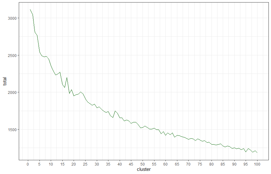
Using The Elbow Method To Identify The Optimal Number Of Clusters

Now we’ve got our graph, we need to use a bit of human intelligence to identify our number of clusters. It’s not perfect, and that’s why other models exist, but I hope this is a good start for you.

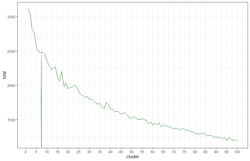
When we look at these charts with the Elbow Method, we’re looking for the point that the chart curves and drops down sharply. The point at which additional clusters become less useful. From looking at the chart below using my dataset, we can see that seven clusters is the point at which we should stop adding extra clusters.

Now we’ve identified k and broken our terms out into clusters, now we need to match it back to our original dataset and name our topics.

From the piece of analysis above, we can see that the optimal number of clusters on this dataset, our k, is seven. Now we need to run the following commands to match them back to our original dataset:

kmeans7 <- kmeans(corpusCleaned, 7)

This is fairly self-explanatory, I hope, but essentially what we’re doing here is creating a new variable called kmeans7 (change it to whatever you like), telling R to use its base kmeans command on our corpusCleaned variable and to use it on the number of clusters we’ve identified. You can obviously adapt this to whatever number of SEO keyword or topic clusters your analysis identified using your own datasets.

Finally, you’ll want to turn this into a clean data frame. You can do that like so:

kwClusters <- as.data.frame(cbind(queries$Query, kmeans7$cluster))

names(kwClusters) <- c("Query", "Cluster")

Now your original keywords are in a data frame with their assigned cluster in the next column.

Now your original keywords are in a data frame with their assigned cluster in the next column and the columns are named “Query” and “Cluster”, keeping them consistent with our main dataset.

From here, we’ll want to get those clusters assigned to our main dataset. Dplyr from the Tidyverse has a really handy left_join function which works a bit like Excel’s Index Match and will let you match this easily.

queries <- left_join(queries, kwClusters, by = "Query")

Again, you’ll need to adapt your variables to fit your datasets, but this is how it’s working with my particular example

What Can You Do With This?

There’s a lot that can be done with this and today I’m updating this post with a few examples of how to do the different elements I’d just suggested previously.

Explore Your Clusters By Subsetting

The easiest way to get to grips with what’s contained in each cluster is to subset and explore accordingly.

Subsetting is one of the most essential elements of working with large datasets, so it’s definitely worth getting to grips with. Fortunately, R has a number of base functions to let you do just that.

Let’s take a look at our first cluster in isolation:

clusterOne <- subset(queries, Cluster == 1)

Here, we’ve cut down our dataset to only look at cluster one. When you’re subsetting or using other exact matches in R, you need to use the ==, otherwise things can get a bit skewey.

Let’s explore it a little. First, we want to see how many observations (keywords in this case), we have in this cluster. Nice and easy – in fact, in RStudio, you can just look in the Data pane like so:

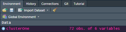
But let’s do it with some code anyway. The nrow function in base R will do that for you.

nrow(clusterOne)

How about if we want to see the number of impressions and clicks from that cluster? We can use the Tidyverse’s summarise function for that:

clusterOne %>% summarise(Impressions = sum(Impressions), Clicks = sum(Clicks))

This will give us an output of the total number of impressions and clicks from that cluster, which can be useful when identifying the opportunity available. Obviously, you can use this for other elements as well. Perhaps you’ve merged some search volume data in, for example, or you want to see what your average position is for this cluster.

Exploring your data in subsets will give you a much greater understanding of what each cluster contains, so it’s well worth doing.

Create Wordclouds By Cluster

Wordclouds are something that always tend to go over well in client presentations, and, although a lot of designers hate them, they’re often a fantastic way to see the most common keywords and terms in your dataset. By doing this by cluster, we’ve got a great way to dig into what each cluster is discussing.

The Wordcloud package for R has everything you need to do this.

Let’s take a look at the queries in my first cluster:

wordcloud(clusterOne$Query, scale=c(5,0.5), max.words=250, random.order=FALSE, 
          rot.per=0.35, use.r.layout=FALSE, colors=brewer.pal(8,"Dark2"))

This will create a wordcloud from that keyword cluster’s query column, give it some pretty colours and present it in the RStudio plots pane. In this cluster’s case, the wordcloud looks like this:

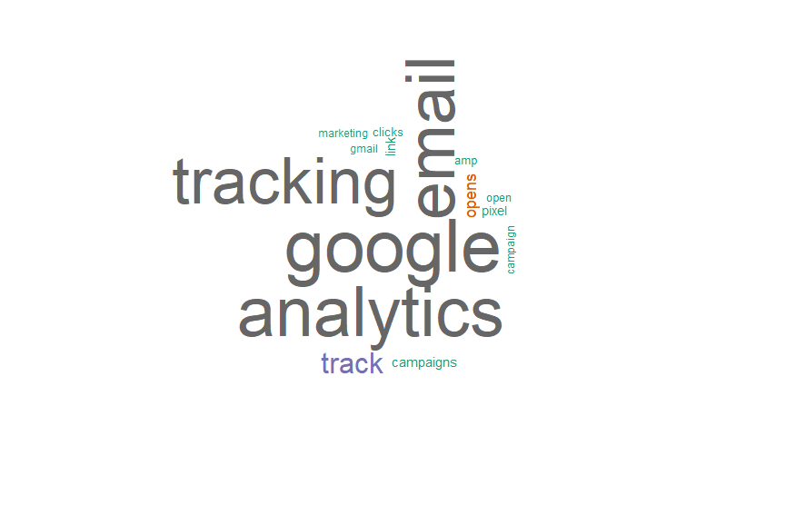
As you can see from here, cluster one of my Search Console data is all about tracking email in Google Analytics.

Wordclouds are a really quick and visual way to explore and identify the topics covered in your keyword clusters and using R instead of a separate tool will help you do that nice and easily without needing to leave RStudio.

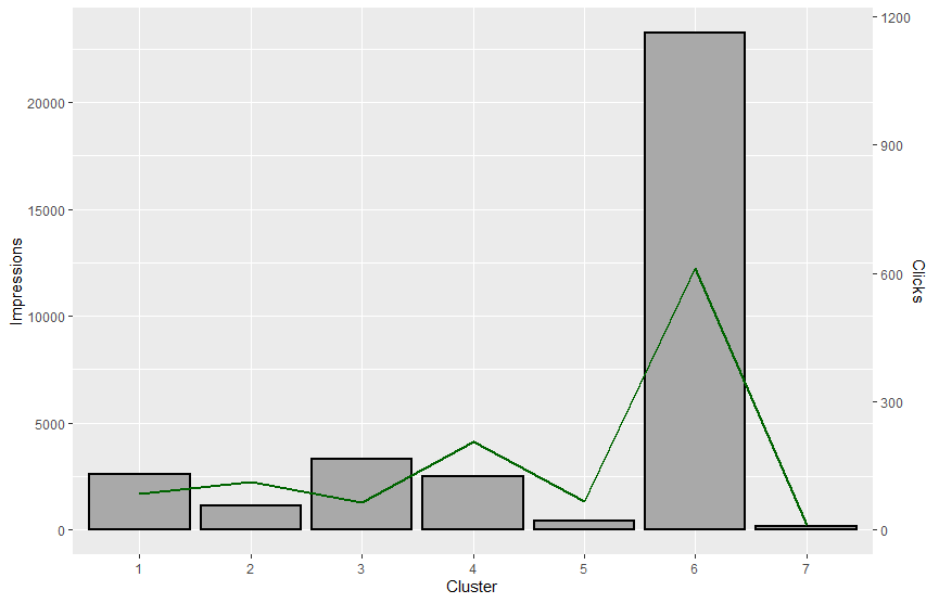
Plotting A Combo Chart With R & GGPlot

The final idea I’m going to run through today is to plot a combo chart where we look at impressions and clicks by cluster. The analyst in me is not a big fan of combo charts since they’re rather flawed, but they are a great way to quickly identify opportunities to improve SEO performance in your keyword clusters. I’m also not very good at making R graphs look pretty, so sorry for that!

Again, you can adapt this to look at a wide variety of different metrics and using the GGPlot package from the Tidyverse gives you a lot of fun graphical avenues to explore.

Firstly, we want to create a dataframe containing a summary of the dataset. You can do that like so with a Dplyr function:

querySummary <- queries %>% group_by(Cluster) %>%
  summarise(Impressions = sum(Impressions), Clicks = sum(Clicks), Avg.Position = mean(Position),
            Avg.CTR = mean(CTR))

Now we have a frame which contains all our keyword clusters with the total impressions, total clicks and the average position and CTR in place, which will be useful for a wide variety of visualisations, not just this example.

The code below will create a column graph with the impressions by cluster and the clicks on a line chart with a secondary axis scaled by 20 to accommodate the differences between the two variables. You can absolutely feel free to change the colours to make it look better.

ggplot(querySummary)+
  geom_col(aes(Cluster, Impressions), size = 1, colour = "black", fill = "darkgray")+
  geom_line(aes(Cluster, 20*Clicks), size = 1, colour = "darkgreen", group =1)+
  scale_y_continuous(sec.axis = sec_axis(~./20, name = "Clicks"))

This will give the following graph:

And there you have it – a really simple introduction to keyword clustering for SEO and some things you can do with it before you start creating your content accordingly.

Wrapping Up

I really hope that this will help some of you that have been wanting to use keyword and topic clustering to better target your SEO but haven’t had the budget for the tools. Everything I’ve talked about here is free to use and, while you might need to do a bit of extra reading to fully get what’s going on, I really hope it’s been helpful.

The most important thing to do with this is to be ruthless. Keep your keyword and topic clusters small and investigate the classifications manually because the wider the base, the less you’ll do with it and the less effective it’ll be.

There is so much that can be done with this that one day, if the world ever goes back to normal, I’ll maybe do a talk on it somewhere, but the key thing to understand is that techniques like this don’t do the job for you, but they do help you do the job a hell of a lot better.

As usual, any questions, shoot me a line on Twitter or through the contact form.

I’ve put the full script below, amend as required.

Until next time.

The Full Keyword And Topic Clustering For SEO R Script

## Install Packages

options(warn=-1)

set.seed(12)

memory.limit(1600000000)

instPacks <- c("tidyverse", "tm", "wordcloud")

lapply(instPacks, require, character.only = TRUE)

## Read Data

queries <- read.csv("Queries.csv", stringsAsFactors = FALSE)

## Prepare Text

dtm <- Corpus(VectorSource(queries$Query))

corpusClean <- function(x){
  
  lowCase <- tm_map(x, tolower)
  
  plainText <- tm_map(lowCase, PlainTextDocument)
  
  remPunc <- tm_map(lowCase, removePunctuation)
  
  stemDoc <- tm_map(remPunc, stemDocument)
  
  output <- DocumentTermMatrix(stemDoc)
  
}

corpusCleaned <- corpusClean(dtm)

## Elbow Method To Find K

kFrame <- data.frame()

for(i in 1:100){
  k <- kmeans(corpusCleaned, centers = i, iter.max = 100)
  kFrame <- rbind(kFrame, cbind(i, k$tot.withinss))
}

names(kFrame) <- c("cluster", "total")

## Visualise Elbow To Find K

ggplot(data = kFrame, aes(x=cluster, y=total, group=1))+ 
  theme_bw(base_family = "Arial")+ geom_line(colour = "darkgreen")+
  scale_x_continuous(breaks = seq(from=0, to=100,by=5))

## Identify Clusters

kmeans7 <- kmeans(corpusCleaned, 7)

kwClusters <- as.data.frame(cbind(queries$Query, kmeans7$cluster))

names(kwClusters) <- c("Query", "Cluster")

## Merge Clusters To Query Data

queries <- left_join(queries, kwClusters, by = "Query")

## Explore Clusters With Subsets

clusterOne <- subset(queries, Cluster == 1)

## Wordclouds

wordcloud(clusterOne$Query, scale=c(5,0.5), max.words=250, random.order=FALSE, 
          rot.per=0.35, use.r.layout=FALSE, colors=brewer.pal(8,"Dark2"))

## Impressions/ Clicks By Cluster

querySummary <- queries %>% group_by(Cluster) %>%
  summarise(Impressions = sum(Impressions), Clicks = sum(Clicks), Avg.Position = mean(Position),
            Avg.CTR = mean(CTR))

ggplot(querySummary)+
  geom_col(aes(Cluster, Impressions), size = 1, colour = "black", fill = "darkgray")+
  geom_line(aes(Cluster, 20*Clicks), size = 1, colour = "darkgreen", group =1)+
  scale_y_continuous(sec.axis = sec_axis(~./20, name = "Clicks"))