R For SEO Part 1: The Basics

The R programming language has lots of benefits for SEOs, but it just doesn’t get as much love in the space as Python. I get it. The barrier to entry is a little higher and there are some things that you can do with Python or other languages that R is just not built for, but when it comes to analysis of chunky datasets or common SEO analytical functions, R can do it just as well as any other language – better in some cases.

R was the first programming language I learned “properly” after self-teaching a few bits of different ones here and there and, although I’m moving more towards focusing on Python and Julia these days for some of the work I’m doing, R will always hold a special place in my heart. With that in mind, I wanted to share a series of posts where I’ll show you just how you can use R for SEO.

How My R For SEO Series Will Work

Over the next eight posts, I’ll be taking you from complete R newbie up to the point where we’re doing serious SEO work, like building a rank checker and dashboard with the language, covering functions, visualisation, replicating Excel formulae and using APIs along the way. If you want to be the first to know when a new entry has dropped, sign up for my FREE email list. No spam, no sales, just updates of new content.

What’s Your Email Address? *

If you are human, leave this field blank.

Δ

While it’s not a completely exhaustive course on R, my hope is that by the end, you’ll have enough of an understanding of the language to use it in your day-to-day SEO work and be able to find answers to any issues you’re having. I’d also absolutely love it if you’d share this series with your network. Over the next few months, I’ll be doing some more stuff for the R community focusing on SEO, so it would be great to have that amplification.

Today, we’re going to be covering the very basics of using R for SEO and future posts will centre around specific elements of the language. I’ll update this post with links to those when they get published as well. Every post will introduce the concepts that we’re discussing and take you through how they work and, at the end, I’ll demonstrate what we’ve learned with an SEO-specific use case.

As always, feel free to use the table of contents below to skip around if you’re looking for a specific area and the code that we use in each section will be compiled into one script and posted here.

OK, let’s get started.

Why Use R?

I’m not going to get into the R vs Python/ SAS/ Matlab/ Julia debate, but I suppose it’s a worthwhile place to start. Just why would we use R, a statistical programming language, in SEO?

Personally, I’ve always loved data and the pattern recognition that comes with its analysis – pretty similar to why I love SEO. I’ve always used data as my secret weapon within SEO and, when I trained as a data analyst, I was keen to make sure I learned to make the skills as transferrable as possible. These days, we’re seeing a lot of analytical programming being used by SEOs, and R is a fantastic way to leverage that.

Ultimately, in SEO, we’re always working with data, sometimes lots of it, and there are situations where the trusty Excel spreadsheet will either not suffice or the size of the dataset will kill your machine, so it’s worth learning R or similar as an additional string to your bow. Think of it as Excel on steroids and you won’t go far wrong.

As languages go, R is a bit on the limited side compared to others. It’s built for statistical analysis and it does that one thing very well, although as you may have seen with my bulk image resizing post, you can make it do plenty of other things as well. For pure data analysis, there aren’t many languages that are better, and the range of packages, visualisation options and, in my opinion, the best IDE on the market makes R a great choice for the data-savvy SEO.

Installing R

Now that we’re ready to get started, the first thing we have to do is install the R language on our machine. This is really simple.

Firstly, go to the CRAN site at https://cran.r-project.org/mirrors.html and select the server that’s closest to you.

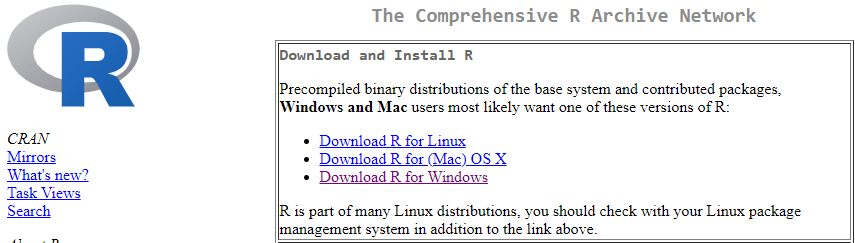
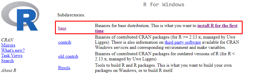
From here, choose the appropriate download for your machine. R is available on Windows, Linux and Mac, and it’s open source, so there’s really no barrier to getting started.

Once your installer has downloaded, install as you usually would any other program. The only change to the installation process I suggest making is unticking “Associate with .Rdata” and .R files. The reason for that is that we’re going to use RStudio for our IDE and we don’t want to just open up the language console every time we double-click on a file.

I generally also recommend only installing the 64-bit version. Using a 32-bit version of the language kind of defeats the object of using this and if you’re still using a 32-bit machine in 2022, you should probably have a serious conversation with yourself or your IT department.

Once everything’s installed, we’re ready to go to the next step: installing RStudio.

Installing RStudio

RStudio is R’s IDE (Integrated Development Environment) and, in my opinion, the best IDE on the market for data analysis, although I do also love PyCharm for working in Python.

An IDE like RStudio lets you write and run your code as well as manage your objects, merge everything you’re working on into specific projects and see your visualisations in one window. They’re essential for any programming work that requires analysis, so it’s great that R has one that’s so good.

You can get RStudio from https://www.rstudio.com/products/rstudio/ – don’t let the paid options scare you, I’ve been using the free one for years and it’s more than good enough for any application.

Installation is just as simple as any other program, but you’ll want to make sure that it’s associating with the relevant file types. If it’s your first installation, select all options. 

OK, now we’re all installed let’s start using R. 

A Quick Tour of RStudio 

The easiest way to show you about how RStudio works is to simply show you how RStudio works, which you’ll find in the image below. 

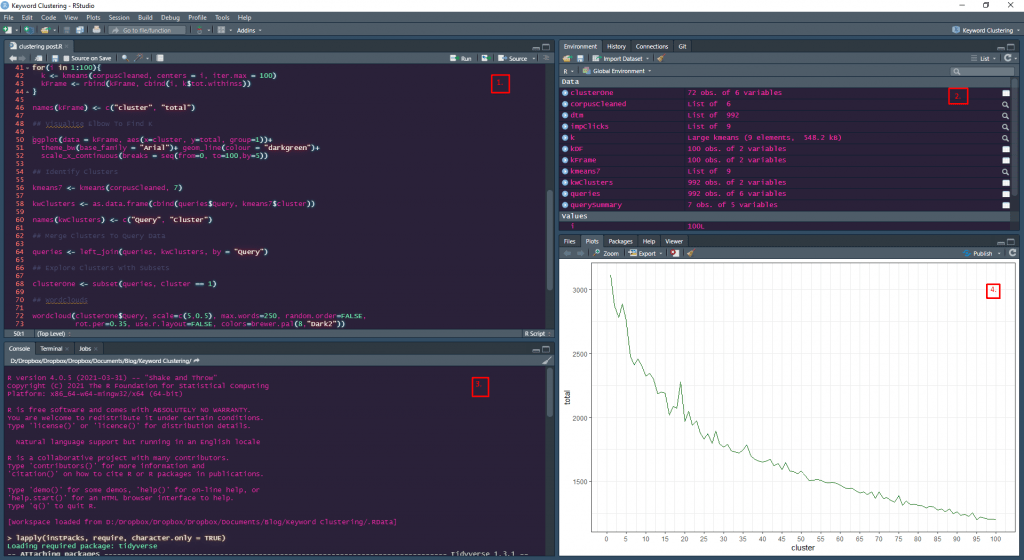
Again, we’re not going fully exhaustive here, but hopefully this screenshot will give you an idea of what’s where. We’ll cover the specific functionality of each section shortly, but here’s a top-line overview: 

1. The Script Window: Where you write and save your code. You can write anything here without breaking anything and it saves down to a .R file, letting you save your code
2. The Environment Explorer: Where you can see the datasets, variables, objects and functions you’ve written into R
3. The R Console: This is where you’ll actually run your code after writing it in the script window
4. The Plot Window: Where you’ll see the graphs you generate. The different tabs also let you see the files in your working directory, the packages you’ve got installed and view help documentation

Now we know what’s where, the best way to get to grips with R is just to start using it, so let’s go. 

Your First RStudio Project 

Before we do anything, we need to create an RStudio project, which will store all our datasets, our code and everything else we’re working on. You should do this with every single piece of work you do with R, just so you can go back to it later. 

As you get a bit more advanced, you may well want to use version control, which I highly recommend. You can read my guide to Git for Data Analysts to get an understanding of how you can use that and what best practices would look like, but we’re not there yet. 

First, create a folder that you’d like to save your first project in. 

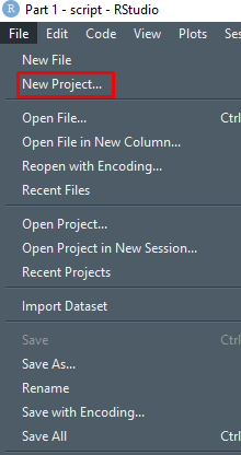
Now in RStudio, click on File and select “New Project” like so. 

Now you’ll want to select “Existing Directory” since we’ve just created that folder. 

Navigate to your project directory and click “Create Project”. 

Finally, click File and “New Script” to give yourself a .R file to write and store your code.

OK, great. Now we’re ready to get cracking on our first R project. But first, we need to get some understanding of how it works.

Datasets And Basic Calculations

Since we’re starting from the very beginning here, we need to start from the actual beginning – creating datasets and basic calculations. Let’s not run before we can walk.

Let’s create our first data frame – essentially, a dataset in its own right.

There are three stages to a data frame: 

1. The name: What we call this variable. It’s always best to choose the most descriptive name you can so you can figure out what it’s doing later
2. The function: This isn’t always essential if your variable is just a number or a string of text, but sometimes, you’ll want to call a function. More on that later
3. The data: What information are we including in this variable? This is where we define it 

Again, we’re only at the basics here, so these aren’t always necessary here, and sometimes as we progress, there will be more elements.

Our First R Dataset

Let’s create and store our first object: 

x <- 2

Seems simple, right? That’s because it is, but let’s break it down anyway. 

• x: The name of our dataset. I know I said to keep your names descriptive, but all shall become clear later 
• <-: The arrow is the most common way of telling R that the name we typed is a dataset name. Some people use the = symbol, which also works fine, but in R, <- is the standard way of doing it 
• 2: The value of our dataset. This will be expanded exponentially later on, but we’re starting at the basics right now 

So, following that, we can tell that our dataset called “x” has a value of 2. 

Paste this into your console window and hit enter, and you should see it in your RStudio Environment Explorer. 

Our First Calculation In R

Now we’ve got our first object, x, with a value of 2, let’s create another one before we start our first calculation in R. 

y <- 3

Now we’ve got a second variable called y with a value of 3. What if we created a new object called z where we try different calculations of the two? 

z <- x+y

As you may have guessed, here we’re adding our x and y datasets and creating a new object called z with the total. 

Try it out. You can just type your dataset name into the R console in RStudio to print the value in the console, or type print(z), whichever you prefer. 

If you used the same values I used for the datasets, you should be given the following in the R console: 

[1] 5

Here, you can see the row number of our output ([1] in this case, since there’s only one row in this dataset), and the value of it. 5, in this case. 

You can do the same thing with other common mathematical calculations: 

• z <- x*y: This will multiply x and y 
• z <- x-y: This will subtract y from x 
• z <- x/y: This will divide x by y 

It’s worth knowing that you can overwrite your dataset names at any time whenever you need to make changes to your code, so you can use the same dataset multiple times, but it’s generally not best practice to do so unless you’ve made a mistake. More on that later. 

But we didn’t start learning R to just do basic calculations, did we? Let’s start using it properly on some real SEO data. 

Of course, in order to do that, we’re going to need some data to work with. Let’s import a spreadsheet and work with that.

Reading CSV Data In R

Since we’re focusing our R learning on SEO, it makes sense for our first project to be using SEO data, so why not use a Google Search Console export? As we go forward, I’ll show you how to get this directly from the API, but that’s another lesson for another time. For now, just do the standard Google Search Console export of your queries. 

This should give you a file called “Queries.csv”. Move that file into your project directory. 

Now we’re going to use a command which you will be using an awful lot with your time in R – read.csv. 

This command reads the contents of a CSV file into your R environment, retaining the structure that you’d see if you opened it in Excel. Let’s see how it works. 

queries <- read.csv("Queries.csv", stringsAsFactors = FALSE)

There it is, your first piece of “proper” R code. Feels pretty cool, right? Put this in your script editor window and, when you’re happy with it, paste it into your console and hit enter. 

You’ll see a dataset called “queries” pop up in the environment explorer in the top right of your RStudio window.

Let’s break it down. As we go through, I’m not going to break down every single command, but this is our first, so it makes sense to.

• queries <-: We’re telling R that we want to call our new dataset “queries”. Again, the “<-“ command is similar to the “=” you’d see in other languages like Python. = does actually work in R, but it’s most common to use <- to define our datasets
• read.csv: The name of our command – in this case, the function to read a CSV file into our environment is helpfully named “read.csv”. Don’t get too used to this, there are some R functions that have me wondering why you’d ever call them that, but that’s part and parcel of any programming language
• (“Queries.csv”,: The name of the CSV file we’re reading in. Don’t forget the quotation marks or to put the full name of the file in
• stringsAsFactors = FALSE): There’s a fantastic article on R-Bloggers about what this does and what you should use it for, but in general, factors are absolutely terrible things and you will almost never want your data to be read in using factors, so I would say for 99% of the occasions you’re reading in CSV data, the stringsAsFactors = FALSE command should be added

And there we have it, we’ve got some data to work with.

One of the key differences between analysing data with code compared to analysing data through Excel is that you can’t actually see it in code compared to looking at a spreadsheet. But not to worry, R has a number of really easy ways to explore and investigate your SEO data.

Basic Data Exploration In R

There are a few key functions that we can use to explore datasets in R: 

• nrow: Tells us how many entries we have in there 
• str: Tells us the structure of the dataset – the headers, the type of data it is and gives us a couple of figures from the top of the dataset
• head: Shows the top results from the dataset 
• tail: Shows the bottom results from the dataset 

There are a few others, which we’ll look at in a second. 

First, we want to see how many rows we have in our dataset. You can just look in the Environment Explorer to the top right like so: 

But if we want to see it in our Console window, we’d type the following: 

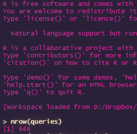
nrow(queries)

This will return the number of rows in our dataset. In my case, it’s given me 646. Your number will almost certainly be different (and probably higher if you spend any actual time working on your site, which I am very bad for).

Now let’s see what the structure looks like. What headers do we have in our dataset? 

To do that, type the following: 

str(queries)

This will return the following output:

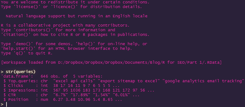
As you can see, we’ve got the following headers in our Search Console dataset: 

• Top.queries: The search terms that people have used to find our website 
• Clicks: The number of times each search term has been clicked 
• Impressions: The number of times each search term has been seen in search results
• CTR: The percentage of clicks to impressions 
• Position: The average position that the search term has been seen in 

This information is obviously really useful to us as SEOs and over the next series of posts, we’ll be looking at how we can use it more.

Head And Tail Investigations In R Datasets 

Now for further investigation, let’s take a look at the top and bottom values of our Search Console dataset using R’s “head” and “tail” functions. 

To see the top of your dataset, in your console, type: 

head(queries)

And to see the bottom of it, type: 

tail(queries)

These will show the top 20 and bottom 20 results respectively, and can be vital in exploring your datasets.

Sum, Average, Max And Minimum Values In R

This is all really useful, but sometimes we just want to see the maximum, minimum, average or total values of a dataset or a variable. Here’s how you do that, using our Google Search Console data. 

Firstly, we need to understand how to focus on a specific variable (similar to a column) in a dataset rather than the dataset as a whole. This is really easy – you simply type your dataset name and add the $ character. If you know the name of your variable, which you can find from the str() command, or RStudio will give you a lovely dropdown menu which will autocomplete. I told you RStudio was great! 

To see the total value of your Impressions variable (similar to running =SUM on a column in Excel), type: 

sum(queries$Impressions)

To see the mean average value of your Impressions variable (similar to using =AVERAGE on a column in Excel), type: 

mean(queries$Impressions)

And if you want to see the median value of your Impressions, you’d type: 

median(queries$Impressions)

Now let’s see what the maximum and minimum values are. We’ll cover this in more detail in part 5 when we start replicating common Excel functions in R. 

max(queries$Impressions)

This will show you the highest number of impressions you’ve had. 

min(queries$Impressions)

And this will show you the lowest number. 

Exploring Data With Summarise In R

Finally, let’s create a summary of our impressions data, so we can see all these values in one go. For bonus points, we’ll create a dataframe of it, so we can review it at any time. 

To use the summarise (summarize if you’re installing in EN-US) function, we’re going to be identifying specific headers from the dataset rather than using it as a whole. To do that, we’re going to use the “$” symbol to call out the specific headers we want to look at, which our str() command will help us find (although RStudio will also autocorrect for us).  

Let’s get a summary of our impressions. 

Type: 

impVals <- summary(queries$Impressions)

This will give you a new variable called impVals (short for Impression Values – remember how I was saying about giving variables memorable names?), which incorporates the following: 

• Min: The lowest number in our range 
• 1^st Qu: The first quartile, or the point at which 25% of the data is cut off in ascending order 
• Median: The middle average value 
• Mean: The average value 
• 3^rd Qu: The third quartile, the point at which 75% of the data is cut off in ascending order
• Max: The highest value in the range 

Summaries can be incredibly useful when exploring data. In fact, it’s quite rare that I don’t have a summary in my R environment of most of the pieces of data I work with, because they’re just so handy to have for reference.

Subsetting Data In R

One of the unfortunate truths of working with data is that most datasets will have a lot of information in them that you don’t want. From irrelevant queries, to numbers too small to be useful, there will be times that you want to just cut information from your dataset, or focus on one specific element. That’s where subsetting comes in.  

Subsetting is a hugely powerful tool for your SEO analysis, so it’s well worth learning how to do it with R. We’ll be using it in the coming articles, so what better time to go through how it works? 

Google Search Console data in particular is a prime candidate for subsetting since you’ll wind up with a lot of random queries in there at times, which are worth cutting out. 

Let’s look at our Google Search Console dataset that we’ve already read into our environment. From the summary in my example, we can see that there are a lot of queries that have only had one impression. We can say that we don’t want to include these in our analysis. 

What we’re going to do here is to create a new dataset based on our queries dataset, but cutting out any queries with 10 or fewer impressions. This would take a few steps to do in Excel, but thankfully, we can do it in one line with R. 

queriesSub <- subset(queries, Impressions >=20)

That’s it. Let’s break it down:

How The Subset Command Works 

The subset command above works as follows: 

• queriesSub <-: Our dataset’s name
• subset(: We’re telling R that subset is the function we want to use 
• queries: The name of the dataset we’re working on (queries in this case, the Search Console data we imported earlier) 
• Impressions: The variable within the dataset that we want to focus on (Impressions in this case) 
• >=20): We’re telling R that we want to only include queries that have 20 or more impressions – >= means “Greater than or equal to”. Don’t forget your closing bracket 

Now we have a new dataset called queriesSub without as many junk impressions included. You can also use a range of other commands with subsets, such as <= (less than or equal to), == (exactly equal to – don’t forget the double = symbol for an exact match) and more. You can also subset based on specific text strings and much more. We’ll cover more of that in future pieces. 

Exporting To CSV With R

As you work further through your analysis, there will certainly be times that you need to export your data to CSV. Perhaps you need to share it, maybe you want to use the information in another tool or spreadsheet, whatever. The point is, you’ll need to do it. Fortunately, this is very simple in R using the write.csv command. 

Let’s export the subset we created of queries with more than ten impressions.  

write.csv(queriesSub, "queriesSub.csv")

Nice and simple. Now if you look in the files pane in RStudio, you’ll see your new file, and it’ll be in your project directory too, all ready for sharing or importing into something else.  

Let’s break it down.

How Write.csv Works In R

Write.csv is a base R command, meaning you don’t need any extra packages or dependencies to run it. It works as follows:

• write.csv(: Here, we’re telling R that we want to use the write.csv command and export a specific dataset to the csv format. Others such as write.txt are available if you need a text file export, they all work largely the same way 
• queriesSub: We’re saying that the dataset that should be written to CSV is our queriesSub dataset. As you do more with R, you’ll be changing this a lot, but it’s a nice and simple command 
• “queriesSub.csv”): Here, we’re naming the file that we want to export to. Nice and simple, but don’t forget the quote marks 

There we go. Now you know how to do some of the basics in R, which will hopefully help you elevate your SEO analysis game.

And We’re Done

Thanks for working your way through the first instalment in my R for SEO series. Hopefully now you’ve got a grasp of the basics of R and you’re all ready for the next piece where we’ll be covering Packages, Google Analytics and Google Search Console data. 

This is where you’ll start to see it coming together, so I really hope you’ll join me next week. 

If you’re going to be along for the ride, thank you. Sign up for my mailing list below and you’ll get an email notification of when it gets published and you can work through the exercises at your leisure, and if you have any questions, hit me up on Twitter.

Until next week.

Our Code From Today

# First Variables

x <- 2

y <- 3

# First Calculations

z <- x+y

print(z)

z <- x*y

z <- x-y

z <- x/y

# Read In Search Console Data

queries <- read.csv("Queries.csv", stringsAsFactors = FALSE)

# Explore Search Console Data

nrow(queries)

str(queries)

head(queries)

tail(queries)

## Further Exploration

sum(queries$Impressions)

mean(queries$Impressions)

median(queries$Impressions)

max(queries$Impressions)

min(queries$Impressions)

## Summary

impVals <- summary(queries$Impressions)

# Subsetting

## Subset Queries To 10 Or More Impressions

queriesSub <- subset(queries, Impressions >=10)

## Subset Queries To 50 Or Fewer Impressions

queriesSub <- subset(queries, Impressions <=50)

## Subset Queries To Exactly 50

queriesSub <- subset(queries, Impressions ==50)